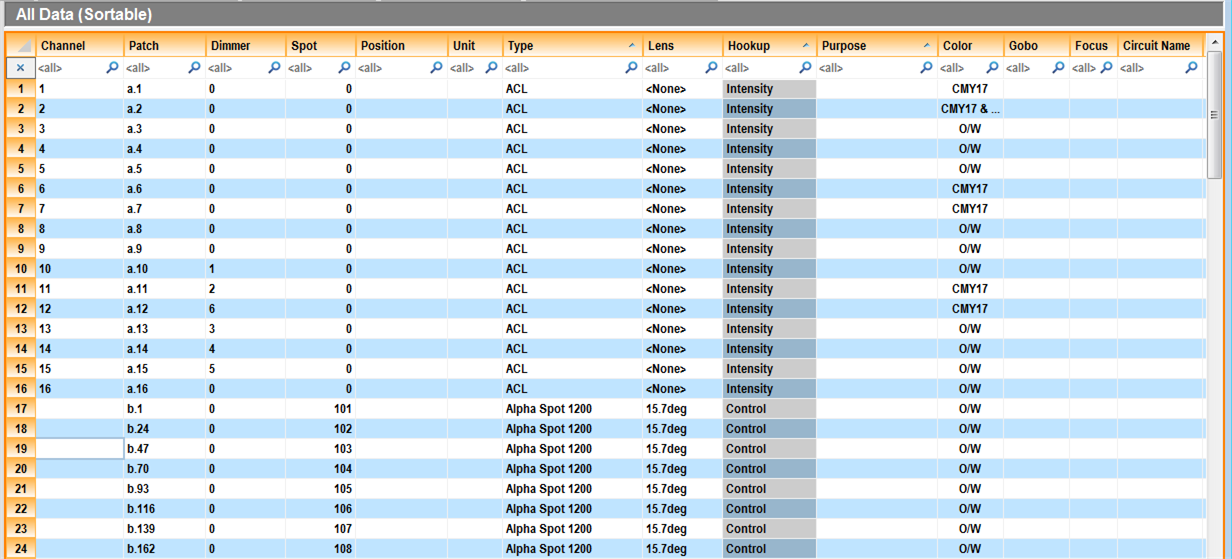
Spreadsheets
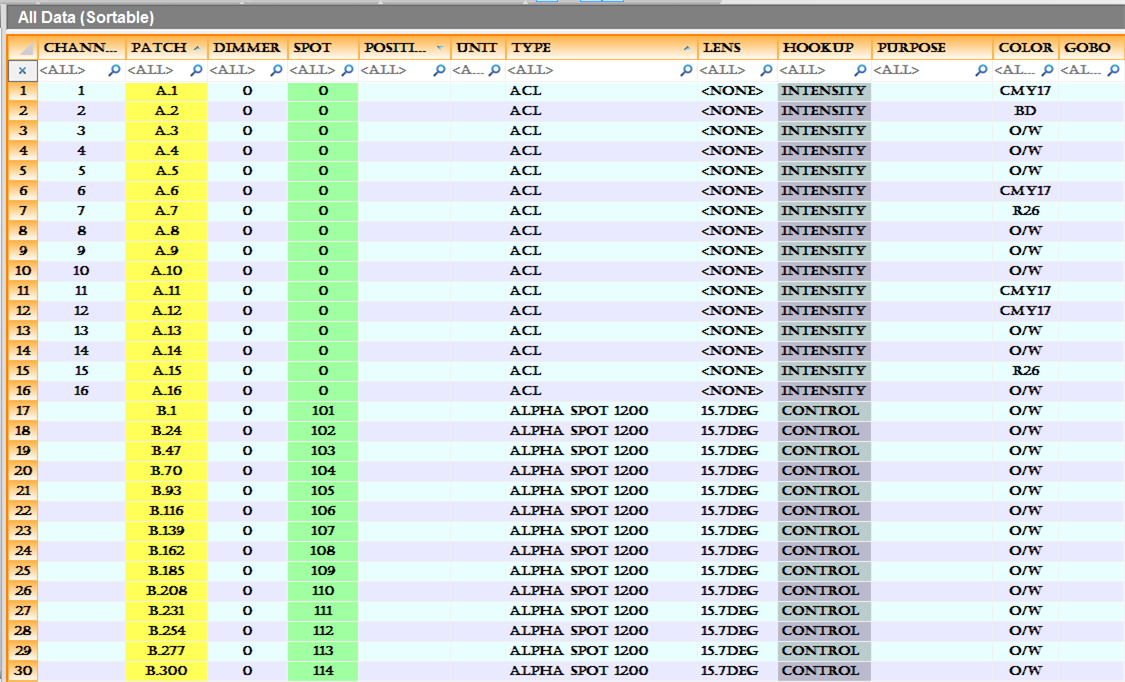
The DATA mode displays your fixture information
in spreadsheet format. WYSIWYG compiles many spreadsheets that are accessible
from the columns shortcut bar. All of these spreadsheets contain the same
information, but are sorted and filtered differently. Each column in the
spreadsheet represents one fixture attribute. The following information
is compiled.
DATA mode also displays your rigging point
information in spreadsheet format. For more information on rigging point
spreadsheets, see Rigging
point spreadsheet.
Data fields
Notes:
- Data fields identified with an asterisk (*) are
non-editable fields.
Spot - This is an assigned
identifier number usually used for automated fixtures. A spot number is
required for automated fixtures when using AutoFocus.
Channel -
This is the assigned control channel number you will use at your control
console to control the fixture. For moving lights, the channel number
recorded in WYSIWYG is the starting channel number.
- To use the AutoFocus feature properly, for most
consoles, the Channel number that appears here must match the starting
number of the fixture's DMX address. For example, if your Mac 500
is patched to universe "A" at address 101 (i.e., the Patch
field reads "A.101"), you must enter the number 101 into
this fixture's Channel field. This must be done manually because the
automatic sequential numerical data entry method does not apply in
this case. For details, see To
input sequential numerical data.
- Data fields identified with an asterisk (*) are
non-editable fields, and can be identified on the spreadsheet as tinted,
if you enable the “Non-Editable Column Tint” option from the View Options or the Data
Spreadsheets toolbar.
Data fields
- Channel - The assigned
channel of the fixture.
- Patch
- This is the fixture’s assigned DMX channel number. This field
is mandatory for simulation activity in LIVE mode. One show can have
multiple DMX universes. A patch entry must be notated universe.#,
where universe is a
letter, number, or other label identifying the universe or output
and # is the DMX channel number. For example, “A.1” or “Dim.26”.
- Dimmer
- This is the assigned dimmer number.
- Spot - The spot ID
of the fixture.
- Position
- This is the hanging position for the fixture. Positions must
be entered in the Position Manager.
- Unit -
The unit number identifies the fixture’s location on its respective
hanging position.
- Type
- This is the fixture name.
- Lens -
This is the lens type.
- *Hookup -
This identifies the component of a multi-circuit fixture or other
device, such as a scroller (for example, intensity, control).
- Purpose -
The purpose is a custom note that is most commonly used to describe
how this fixture is being used in your show. For example, “SL Side”,
“Diagonal Backs”. Purpose is an attribute of the fixture. It is not
possible to assign multiple purposes for multi-circuit fixtures.
- Color -
This is the assigned gel color number or scroller identification.
- Gobo
- This is the assigned gobo number.
- Focus -
This is the fixture’s focus position.
- Circuit Name - This is an identifier
note for the circuit box or multi-cable.
- Circuit Number - This is the assigned
circuit or multi-cable tail number.
- Mode - This is the
fixture’s mode setting.
- Fixture Options -
This is information on the fixtures options, e.g. the, reserved channels,
lamp info, etc.
- *Wattage
- This is the wattage in watts of the lamp.
- Lamp Type - This is the lamp type.
- *Offset -
This field identifies the fixture’s location on the hanging structure.
It is a distance measurement referencing the pipe’s end or center
point or another point as specified.
- *X - This field indicates
the X coordinate of the fixture’s position.
- *Y - This field indicates
the Y coordinate of the fixture’s position.
- *Z - This field indicates
the Z coordinate of the fixture’s position.
- Pan -
A focus attribute measured in degrees, defining the positioning of
the fixtures yoke.
- Tilt -
A focus attribute measured in degrees, defining the positioning of
the fixture within the yoke.
- Spin -
A focus attribute measured in degrees, defining the fixture’s yoke
positioning in relation to the hang structure where 0 is down-hung,
90 is side-hung, and 180 is over-hung for example.
- *Weight -
This is the fixture’s weight. A fixture’s weight can only be modified
through the Library Browser.
- Notes
- This is a custom notes field.
- *Footnotes
- This feature is currently disabled.
- *# of Data Channels - This is the
total number of DMX channels required by the fixture.
- *# of Color Frames - This is the
number of color frame slots that the fixture has.
- *#
of Lamps - This is the number of lamps required by the fixture.
- *Circuit Type - This describes what
type of device the unit should be plugged into, for example, regular
dimmer, scroller power supply.
- *Model
- This is the fixture type.
- *Cost -
This is the fixture’s cost or rental cost. This field is used to estimate
a show budget. A fixture’s cost can only be modified through the Library
Browser. For more information on setting costs, see Data
tab.
- *Status -
This is the fixture’s status relative to your drawing. If the fixture
is HUNG it is in your drawing. If a fixture is UNHUNG, it is in the
flight case. In fixture count reports, all fixtures are counted regardless
of their status (unless a filter is applied).
- *Console -
This identifies which console is controlling the fixture. This field
references the binding settings in the device manager in LIVE mode.
- Layer
- This field indicates which layer the fixture is drawn on.
- *Tag -
This is an internal code used for importing and exporting data to/from
third party programs.
- *Owner
- This feature is currently disabled.
- Manufacturer - This
field indicates the manufacturer of the fixture.
- Notes2 – Additional
column for notes.
- Notes3 - Additional
column for notes.
- Notes4 - Additional
column for notes.
- *RotX - The rotation
of the fixture on the X axis.
- *RotY - The rotation
of the fixture on the Y axis.
- *RotZ - The rotation
of the fixture on the Z axis.
- *Patch Address -
When a patch is specified for a fixture/accessory, this column just
displays the starting address.
- *Patch Universe -
When a patch is specified for a fixture/accessory, this column just
displays the Universe it is patched on.
Working in the spreadsheet
Data
may be entered in a number of ways within the WYSIWYG file. The plot can
be created, and then edited, or the data may be entered in a spreadsheet,
and then placed on the plot. Any entries or changes are reciprocated throughout
the file; changes made in DATA mode will be updated in CAD mode and vice
versa.
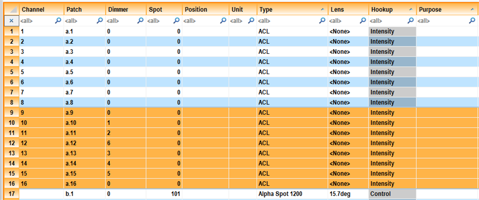
Selection
Standard selection functionality is offered
in the > .
Selected cells are highlighted in orange.
- To select one cell,
just move your mouse over it and click. You will notice a blue outline
appears around the cell.
- To select multiple cells,
select your starting cell and either drag the mouse in any direction,
or while holding the SHIFT key
down, use the arrow buttons on the keyboard.
- To select non sequential
cells, hold down the CTRL button
and click with your mouse on the desired cells.
- To select an entire row,
click on the row header (i.e. The left-most column which has the row
numbers).
To add or modify data
Select a cell, and type the desired value
in the appropriate cell. Notice that some cells accept text (e.g. Channel
column), so you click on them and start typing text. Some cells will display
a drop-down list when they are selected, so you can choose your data from
the drop-down list or type the desired option (e.g. Lens column).
The Spreadsheet has built in intelligence,
and will not accept invalid data entry. For example, you cannot enter
non-numerical data in the Channel column, (it will display an error message).
Columns that are read-only or non-editable
cannot be modified from the Spreadsheet. These columns may be tinted slightly
darker for easy identification from the View Options.
Entering the same
data into multiple cells
You can enter the same information to multiple
cells at the same time by selecting a series of cells, typing your text
in the first cell selected, and then pressing the ENTER button.
You can also delete data in multiple cells at the same time by selecting
the cells, and then pressing the DELETE
button.
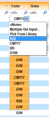
When entering data in some columns (such
as Color and Gobo), a drop-down list will appear displaying some options
to help you enter the data into the cell(s). For the Color column, for
instance:
- <None>: Select
this option if no color is desired.
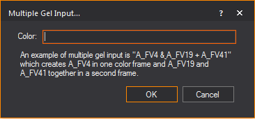
- Multiple Gel Input:
This option displays a dialog box where you can enter multiple gel
manufacturer catalog codes for one fixture
- Pick from Library:
This opens the Library Browser and
you can preview colors in the Gel Library
- List of previously used
gels in your file: For your convenience all previously used
gel color codes are displayed; click on the one you wish to use.
To input sequential numerical
data
If you are entering sequential numerical
values for a field such as Channel or Spot, you can use incremental data
entry to facilitate your work. WYSIWYG will calculate the next available
value based on the number of required channels for the previous fixture.
- In a column, select a series of fixtures to enter
incremental data, by using a selection method such as click and drag.
- Enter in the first cell the starting value of
the data, and then a plus sign ( + ).
Example: If
the first channel in the selected fixtures should be 101, enter “101 +” and then press ENTER.
To assign sequential patch to fixtures
If you are assigning a sequential patch
for a list of fixtures, you can use incremental data entry to facilitate
your work. WYSIWYG will calculate the next available value based on the
number of required channels for the previous fixture.
- Select the fixtures you want to patch sequentially.
- In the first cell type “UniverseName.
Starting Address +”
Example: “F.1 +”
Note: You
can skip channels between the patching of one fixture to the next. To
specify the number of channels that should be skipped, add that number
to the end of the equation “UniverseName . Starting
Address + [# of channels to skip between patching]”.
Example: “F.1 + 4”
- Hit Enter.
Result: The
selected fixtures are automatically sequentially patched.
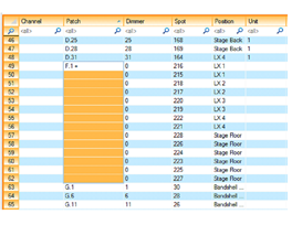

Fixtures selected for multi-fixture sequential
patching. The example used is "F.1 +". |
After performing
the multi-fixture patching command, the fixtures are patched sequentially. |
To choose a new
value
- Select the appropriate cell.
- If values are available, there will be a drop-down
arrow in the cell. Click the drop-down arrow to display the list of
available values.
- Select the value from the drop-down list.
Result: The
cell changes to the selected value.
Inserting
fixtures in data mode
Any fixtures inserted in DATA mode are
assigned the status “unhung” and are placed in the Flight Case. The Flight
Case allows you to drag and drop “unhung” fixtures onto your drawing.
For more information about the Flight Case, see The
Flight Case.
To insert fixtures in data mode
- Click the Fixture tool
on the Data toolbar.
 The Fixture
button.
The Fixture
button.
- Navigate to the desired fixture.
- In the Multiple
box, type the number of fixtures of that type required.
- Click Insert.
Result: The
fixtures are inserted below the last entry in the spreadsheet.
Tip: If you
have a shortcut created for the desired fixture, you can right-click on
the shortcut and choose or .
Inserting
positions in data mode
A position cannot exist in WYSIWYG unless
it is recorded in the Position Manager.
You can if you type a new value into the position field of a fixture,
the Pick a value from the list dialog
box is automatically displayed. This is because a position cannot exist
in WYSIWYG unless it is recorded in the Position
Manager. You can select from the list of positions that already
exist or you can click menu to open
the Position Manager to create a new
position.
If you are making this change to a fixture
that was previously hung on a different position, that fixture will be
unhung and sent to the Flight Case under
its new position field. From there, you can drag it back onto the drawing.
If the position does not yet exist in the
drawing, you must draw a hang structure and assign it the appropriate
position name before you will be able to hang the fixture again. For more
information on drawing hang structures, see Hang structures.
For more information on drawing items from
the Flight Case, see Entering
and modifying objects in the Flight Case.
Inserting color in data mode
To insert color in data mode
- Click in the color field of the fixture for which
you want to assign color.
- Click the drop-down list in the cell and select
either , , or .
Note: If
you know the catalog code for the gel, you can type the gel code in the
cell to choose it. For example, if you want Rosco's "Roscolux Light
Red" gel, type "R26" in the cell and hit ENTER.
Rosco's "Roscolux Light Red" gel will be selected.
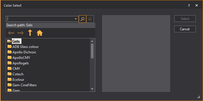
- Use to
select a color among those you have already used in your plot. Selecting
this option will bring up the Color Select
window where you can locate the color you want from a library.
- Use if
you already know the color that you want to assign (for example, R54,
L112, and so on). Selecting this option will bring up the Multiple
Gel Input... window where you can enter the color you
want.
WYSIWYG accommodates multiple color entries
for one fixture as follows:
- “Color1 & Color2” yields two color frames
with one gel in each.
- “Color1 + Color2” yields one color frame with
two gels in it.
- “Color1 / Color2” yields one color frame with
one split gel in it.
Customizing spreadsheets
There are different ways to sort and view
your data. You can modify a spreadsheet to suit your needs. Customizing
a view allows you to change how the data is displayed and sorted.
To
modify a data sheet
- From the menu,
choose .
Result: The
View Options window appears.
Tip: You can
also click the View Options tool on
the Standard toolbar.
 The
View Options button.
The
View Options button.
Note: You
can also right-click on the Spreadsheet shortcut and select .
- In the General tab,
specify how the data sheet will be displayed.
- In the Data Options tab,
specify the information that will be displayed in the data sheet.
- Click OK.
General tab
Options on the General
tab affect the current data sheet.
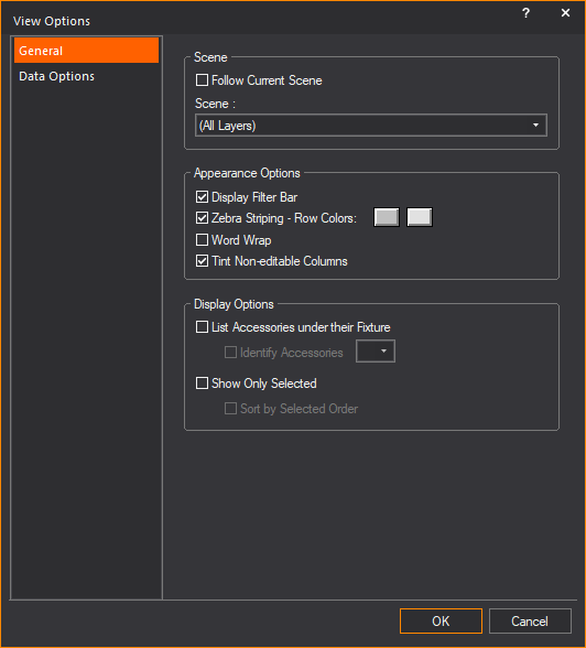
Scene
- Follow Current Scene:
Select this checkbox to use the currently selected scene. Clear and
select a different scene from the Scenes drop-down
list.
- Scene: Name of
the Wireframe view.
Appearance Options
- Display Filter Bar:
Select this checkbox to display filters below the headings of each
column.
- Zebra Striping - Row Colors:
Select this checkbox to display rows in two alternating colors. Click
the Color Select boxes to select the colors for each row.
- Word Wrap: Select
this checkbox to automatically wrap the text in every cell.
- Tint Non-editable Columns:
Select this checkbox to highlight the columns with non-editable data.
Display Options
- List Accessories under
their Fixture: Select this checkbox to display the list of
accessories added to the fixtures in rows that follow after.
- Identify Accessories:
Select this checkbox and select the symbol that identifies the listed
accessory.
- Show Only Selected:
Select this checkbox to display only the fixtures that are selected
in CAD.
- Sort by Selected Order:
Select this checkbox to display the selected fixtures according to
the order of selection.
Data Options tab
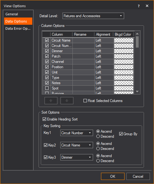
Detail Level
- Fixtures and Accessories:
Select this drop-down menu to display the details of fixtures and
accessories in the spreadsheet.
- Fixtures: Select
this drop-down menu to display the details of the fixtures only on
the Spreadsheet.
Column Options
- Column: Use the
column table to specify column display and order of appearance.
- To change the location of a column in the spreadsheet,
highlight the appropriate column heading in the Columns box,
and then click the Up or Down button.
- To hide a column from your view, clear the checkbox
beside it.
- Rename: Type a
new name in the Rename column to rename the title of the column.
- Alignment: Click
the drop-down list in this column and select the text alignment to
either Left, Center, or Right.
- Bkgd Color: Click
the Color Select box in this column to change the background color
of the column. This can be used to highlight important columns in
your spreadsheets.
- Float Selected Columns:
Select this checkbox to undock the selected column in the spreadsheet.
Sort Options
- Enable Heading Sort: Select
this checkbox to enable the ability to sort the spreadsheet by clicking
on the Column Headings. When you click on a column heading, it becomes
the new Key 1 sort parameter, and the existing sorting options propagate
down to Key 2 and Key 3. Clicking on the same column heading again
will switch the sort from ascending to descending, and vice versa.
- To specify how entries should be sorted, choose
the desired column headings in the Key 1,
Key 2, and Key
3 drop-down lists. When fixtures have the same value in
the first sort key, the spreadsheet is then sorted by the values of
the second sort key.
- Click Ascend or
Descend to sort the criteria in
ascending or descending order, respectively.
- Select the Group By checkbox
to group the spreadsheet into sections, one section for each value
in the Key 1 field.
Font options
To display the Spreadsheet with your preferred
font settings, right-click on the Spreadsheet and select . Choose your preferred font, style, color, size, and script,
and click OK. The text in the Spreadsheet
is now displayed with your new font settings.
Column heading
Some column options are also listed if
you right-click on the column heading.
- : Hides
current column (will not be displayed)
- :
A convenient way to show all columns
- : Since
clicking on the column heading will re-sort the spreadsheet if this
option is enabled, the Select Column option offers an easy way to
select the column.
- :
A convenient way to enable/disable the Column Heading sort option.
- : The
selected column and all the columns to the left of it will freeze
and always visible when scrolling over horizontally to the right.
- :
The selected column will automatically resize so that all text is
visible.
- :
All the columns will automatically resize so that all text is visible.
Filter
bar
When enabled, the Filter Bar appears on
the first row of the Spreadsheet. The Filter Bar offers an easy way to
filter the Spreadsheet or search for exact text or fixtures in any column.
The Filter Bar accepts text in multiple columns simultaneously making
it easier to find a fixture in your Spreadsheet.
Note: To clear
a filter string, you can click the X button
which appears at the right side of the column. If you have multiple filters,
you can click the X button which is
located above the row headers (very far left column with row numbers),
and this clears all filter strings and displays all rows in the Spreadsheet
are displayed again.
To apply a data filter using the filter bar
- In the spreadsheet, click the filter bar on the
column you want to filter.
- Type the specific text,
or select the data from a drop-down menu you
want to filter for.
Result: The
spreadsheet refreshes, displaying only fixtures that meet the filter criteria.
To remove data filters
In the spreadsheet, click the X button
which appears at the right side of the column.
Note: If you
have multiple filters, you can click the X button
which is located above the row headers (very far left column with row
numbers), and this clears all filter strings and displays all rows in
the Spreadsheet are displayed again.
Result: The
spreadsheet returns to its unfiltered state.
Finding
and replacing text in the spreadsheet
Information found in cells can be quickly
accessed and edited using the or the functions. allows
you to search your spreadsheet for words or whole phrases, then selects
the words when found. searches
your spreadsheet the same as Find, but with the additional option to replace
the words.
To find text in the spreadsheet
- From the menu,
choose .
- Alternately, you can use the shortcut CTRL+F.
Result: The
Find dialog box appears.
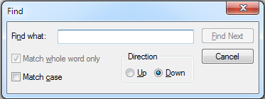
- In the Find what
field, type the text you want to search for.
- Select the Match case checkbox
to search for only words that match the exact case of the text entered
in the Find what field.
- In the Direction section,
select Up or Down to
search the spreadsheet in the chosen direction.
- To search for the next instance of the chosen
text, click Find Next.
To find and replace text in the spreadsheet
- From the menu,
choose .
- Alternately, you can use the shortcut CTRL+SHIFT+H.
Result: The
Replace dialog box appears.
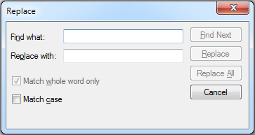
- In the Find what
field, type the text you want to search for.
- In the Replace with field,
type the text you want to replace any found text with.
- Select the Match case checkbox
to search for only words that match the exact case of the text entered
in the Find what field.
- To search for the next instance of the chosen
text, click Find Next.
- To replace found text with the text written in
the Replace with field, click Replace.
- To replace all instances of the found text with
the text written in the Replace with field,
click Replace All.
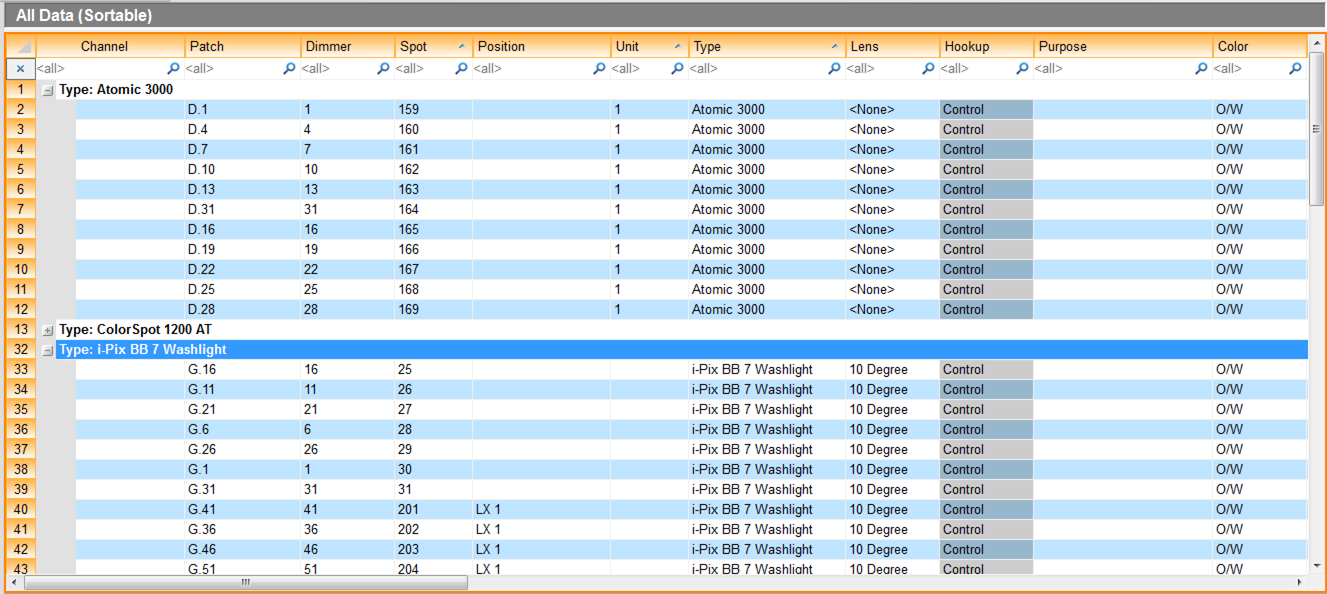
Grouping
the spreadsheet by a column
The group by option is available for the
Column in Key 1 sort, which groups the Spreadsheet into sections. Each
section has a button which expands (+)
and collapses (-) so you can choose if
you wish to displays the rows of data in a group or not.
Freezing
spreadsheet columns
The Freezing Column options allows you
to keep your information in place as you scroll through the rest of the
spreadsheet. This is useful if the spreadsheet is very large and you have
headings that you want to stay in place.
To freeze spreadsheet columns
Right-click a column header, and select
To unfreeze spreadsheet columns
Right-click a column header, and select
Creating a new spreadsheet
To create a new sheet
- On the shortcut bar, click the Columns
tab.
- Right-click on the shortcut bar and choose
Result: The
Enter new Spreadsheet name dialog box appears.
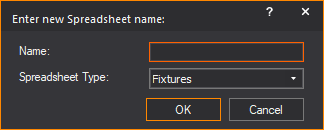
- In the Name box,
type a name for the new spreadsheet.
- From the Spreadsheet Type drop-down
list, click Fixtures or Rigging Point.
- Click OK.
- Scroll to the bottom of the list of Column shortcuts.
Your new spreadsheet name should be at the bottom of the list. Click
on the shortcut to view your spreadsheet.
Note: It may
be easier to clone an existing spreadsheet and modify it than to start
a new one from scratch. See To clone a shortcut for more
details.
Exporting
a spreadsheet
The Spreadsheet can be exported to numerous
formats, in case you wish to use the spreadsheet data from you lighting
show in a different program.
To export a spreadsheet
- >.
- An Export File dialog
box appears for you to enter a file name, and select a file type.
Supported file types include: Microsoft Excel (.xlsx) and (.xls),
HTML (.htm), Comma Separated Values (.csv), WYSIWYG Spreadsheet (.wss)
- Another option in the menu
is to . This option
automatically copies a snapshot of the Spreadsheet into the Worksheet
tab. This is convenient at the end of a project, because a worksheet
can be inserted into a Layout (a Spreadsheet cannot be inserted directly
anymore).
Rigging
point spreadsheet
DATA mode displays information of all your
Rigging Points in spreadsheet format. Each Rigging Point in your plot
appears as a separate row in the Rigging Point spreadsheet, while attributes
appear as columns.
The following attributes appear as columns
in the Rigging Point spreadsheet:
- Name - The name of
the Rigging Point.
- Type - The type of
Rigging Point.
- Bridle - Indicates
(Yes or No)
if the Rigging Point is a bridle sling or not.
- X - The location
coordinate along the X axis.
- Y - The location
coordinate along the Y axis.
- Z - The location
coordinate along the Z axis.
- Capacity - The
maximum load which can be hung from the Rigging Point.
- Load - The actual
load of the object that will hang from the Rigging Point.
- Position - The
name of the Hang Position that the Rigging Point is associated with.
If a Position is not assigned to a Rigging Point from its Properties window,
you can assign the Position from this cell. The Position drop-down
list in the Rigging Point’s Properties window
will match the selection in this cell.
- Notes - Text
that was entered in the Note box
of the Rigging Point’s Properties window.
Text added in this cell will appear in the Notes
box of its Properties window.
- Motor/Hoist Type -
Text field used to enter information about the (type of) Motor or
Hoist associated with the Rigging Point.
- Chain Length -
Text field used to enter information about the required length of
the Motor or Hoist chain.
- Notes 1, Notes
2, Notes 3, and Notes
4 - Text fields used to enter other necessary information
about the Rigging Point.
Tip: You can
rename these columns with more useful titles via the Spreadsheet’s View Options > Data
Options tab. For more information, see Data Options tab.
Rigging Point spreadsheets work the same
as the Spreadsheet with fixture data. Follow the steps in the reference
sections corresponding to the following list of operations.
- To create a new Rigging Point spreadsheet, see
Creating
a new spreadsheet.
- To apply standard functions of a Spreadsheet in
DATA mode, see
Working in the spreadsheet
Customizing spreadsheets
Filter bar
Finding and replacing text in the spreadsheet
Finding and replacing text in the spreadsheet
Grouping the spreadsheet by a column
Freezing
spreadsheet columns
Exporting a spreadsheet
To rename a rigging point in spreadsheet
- On the Rigging Point spreadsheet, click in the
Name cell.
- Type the new name.
Note: The
new name must be unique.
- On your keyboard, press Enter or
click on the spreadsheet off the Name
cell.
Result: The
name of the selected Rigging Point changes.
To rename multiple rigging points in spreadsheet
Follow the steps in the section To input sequential numerical data.
Note: The
selected Rigging Points must have unique names and must end in a number.
You cannot use one name for all the multiple selected Rigging Points.
Result: The
name of the multiple Rigging Points changes.
To change type/bridle/position in spreadsheet
Follow the steps in the section To choose a new value.
Note: When
multiple cells are selected on the Type or Bridle column, you can change
the Type or Bridle values for all the selected Rigging Points.
To change X, Y, or Z of rigging points in spreadsheet
- On the Rigging Point spreadsheet, click in the
X, Y, or Z cell you want to change.
- In the selected cell, type the new coordinate
and related unit symbol or letter.
- On your keyboard, press Enter or
click on the spreadsheet off the selected cell.
Tip: Enter
the coordinates in the same way as you enter coordinates in the Position Tool.
Result: The
selected Rigging Point’s location changes.
Note: Multiple
cells selection.
- When multiple cells are selected on the X, Y,
or Z column, you can change the X, Y, Z location coordinates for all
the selected Rigging Points.
- You cannot enter automatic sequential numbering
on the selected cells in the X, Y, Z columns.
To change capacity and load in spreadsheet
- On the Rigging Point spreadsheet, click in the
cell.
Result: The
unit (lbs, kg, or t) disappears but will reappear after keyboard Enter is pressed.
- In the selected cell, type the new number.
Note: Only
numbers can be entered.
- On your keyboard, press Enter
or click on the spreadsheet off the selected cell.
Result: The
capacity or load of the selected Rigging Point changes.
Note: Multiple
cells selection.
- When multiple cells are selected on the Capacity
or Load column, you can change the Capacity or Load values for all
the selected Rigging Points.
- You cannot enter automatic sequential numbering
on the selected cells in the Capacity and Load columns.